Shape formation using Kilobots
Kilobots are low cost robots designed at Harvard University's Self-organizing Systems Research Lab. Though the Kilobots are low-cost, they maintain abilities similar to other collective robots. These abilities include differential drive locomotion, on-board computation power, neighbor-to-neighbor communication, neighbor-to neighbor distance sensing, and ambient light sensing. Additionally, they are designed to operate such that no robot requires any individual attention by a human operator. This makes controlling a group of Kilobots easy, whether there are 10 or 1000 in the group.

In this project, we designed an algorithm for Kilobots to collaboratively form a given shape. A finite state machine based framework was utilized to breakdown the problem into two essential components. The first component comprised of an orbiting algorithm to allow Kilobots to reach their desired location, and the second, a localization mechanism to identify its relative position. Interested readers are referred to the report below for more details.
Specifications of a Kilobot
The functional specifications of a Kilobot are as follow.
- Processor: ATmega 328p (8bit @ 8MHz)
- Memory:
- 32 KB Flash -- used for both user program and bootloader
- 1KB EEPROM -- for storing calibration values and other non-volatile data
- 2KB SRAM
- Battery: Rechargeable Li-Ion 3.7V, for a 3 months autonomy in sleep mode. Each Kilobot has a built-in charger circuit which charges the onboard battery when +6 volts is applied to any of the legs, and GND is applied to the charging tab.
- Charging: Kilobot charger for 10 robots simultaneously
- Communication: Kilobots can communicate with neighbors up to 7 cm away by reflecting infrared (IR) light off the ground surface.
- Sensing: One IR sensor and one light sensor
- When receiving a message, distance to the transmitting Kilobot can be determined using received signal strength. The distance depends on the surface used as the light intensity is used to compute the value.
- The brightness of the ambient light shining on a Kilobot can be detected.
- A Kilobot can sense its own battery voltage.
- Movement: Each Kilobot has 2 vibration motors, which are independently controllable, allowing for differential drive of the robot. Each motor can be set to 255 different power levels. The movement happens via stick and slip mechanism.
- Light: Each Kilobot has a red/green/blue (RGB) LED pointed upward, and each color has 3 levels of brightness control.
- Software: The Kilobot Controller software (kiloGUI) is available for controlling the controller board, sending program files to the robots and controlling them.
- Programming: C language with WinAVR compiler combined with Eclipse or the online Kilobotics editor (Kilobotics Editor)
- Dimensions: Diameter: 33 mm, height 34 mm (including the legs, without recharge antenna).
Hardware/Software Requirement
The required hardware and software to use the board and develop programs are described below.
Required Hardware
- Computer with a USB port
- Kilobot robot
- Over-head controller (OHC)
- Kilobot charger
Required Software
To start programming the Kilobot with the new version from Kilobotics, we have two solution.
- Online editor: Kilobotics Editor
- Install WinAVR and Eclipse to compile the whole library on your computer: Setup Guide
We used the online editor for this project.
Over-head Controller
To make a robot scalable to large collective sizes, all the operations of the robot must work on the collective as a whole, and not require any individual attention to the robot, such as pushing a switch or plugging in a charging cable for each robot. In other words, all collective operations must be scalable.
In the case of Kilobots, instead of plugging in a programming cable to each robot in order to update its program, each can receive a program via an IR communication channel. This allows an overhead IR transmitter to program all the robots in the collective in a fixed amount of time, independent of the number of robots.
Establishing Communication Between Two Kilobots
Here, we will use the ability of two Kilobots to communicate with each other. We will allocate one Kilobot to be the speaker and the other Kilobot to be the listener.
Speaker
The objective of this part is to broadcast a fixed message and blink magenta when we transmit. Here we introduce the message_t data structure and the kilo_message_tx callback.
- A Kilobot uses IR to broadcast a message within an approximately circular radius of three body lengths.
- Multiple robots packed closely together will interfere with the IR signals. So the Kilobots use a variant of the CSMA/CD media access control method to resolve the problems with interference.
Step 1: Declare a variable called transmit_msg of the structure type message_t and add the function message_tx() that returns the address of the message we declared (return &transmit_msg;).
message_t transmit_msg;

    message_t *message_tx() {
        return &transmit_msg;
    }
Step 2: We will register this "callback" function in the Kilobot main loop, and every time the Kilobot is ready to send a message it will "interrupt" the main code and call the message_tx() to get the message that needs to be sent.
Step 3: Use the setup() function to set the initial contents of the message and compute the message CRC value (used for error detection) through the function message_crc(). The code below shows how to initialize a simple message.
void setup() {
        transmit_msg.type = NORMAL;
        transmit_msg.data[0] = 0;
        transmit_msg.crc = message_crc(&transmit_msg);
    }
Step 4: Now we will add some more code so that we can have the LED blink whenever the robot sends a message out. To do this, we will declare a variable (often called a "boolean flag") called message_sent. We will set this flag inside a function called message_tx_success(), which is another callback function that only gets called when a message is successfully sent on a channel. Then we will clear this flag in the main loop where we will blink an LED to indicate that a message was sent.
// At the top of the file, declare a "flag" for when a message is sent
    int message_sent = 0;

    // Add another function definition after your message_tx function
    // (note that "void" means the function doesn't return any value)

    void message_tx_success() {
       message_sent = 1;
    }
Step 5: Then, in our program loop, write code to do this:
// Blink LED magenta when you get a message
    if (message_sent == 1) {
        message_sent = 0;
        set_color(RGB(1,0,1));
        delay(100);
        set_color(RGB(0,0,0));
    }
Step 6: Finally, we must register our message transmission functions with the Kilobot library as follows:
int main() {
        kilo_init();
        kilo_message_tx = message_tx;
        kilo_message_tx_success = message_tx_success;
        kilo_start(setup, loop);

        return 0;
    }
Listener
The objective of this part is to blink yellow when a new message is received and introduce the kilo_message_rx callback to store incoming messages.
Step 1
First, declare a variable rcvd_message of type message_t to store any new incoming messages and a boolean variable called new_message to indicate that a new message has been received.
int new_message = 0;
    message_t rcvd_message;

    void message_rx(message_t *msg, distance_measurement_t *dist) {
        rcvd_message = *msg;  // Store the incoming message
        new_message = 1;      // Set the flag to 1 to indicate that a new message arrived
    }
Step 2
Check the flag in the program loop to see if a new message has arrived. If a new message has arrived, we will blink the LED yellow and clear the flag.
void loop() {
        // Blink LED yellow when a message is received
        if (new_message == 1) {
            new_message = 0;
            set_color(RGB(1,1,0));
            delay(100);
            set_color(RGB(0,0,0));
        }
    }
Step 3
Modify the main section to register the message reception function with the Kilobot library as follows:
int main() {
        kilo_init();
        kilo_message_rx = message_rx;
        kilo_start(setup, loop);

        return 0;
    }
Results and Demonstration
For this task of establishing communication between two Kilobots, the communication protocol CSMA/CD has been followed. Thus, the speaker Kilobot will first sense and then transmit.
According to the Kilobotics website, by default, every Kilobot attempts to send a message twice per second.
Orbiting of Kilobots
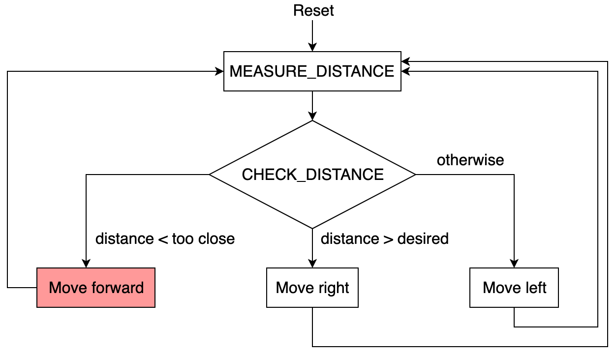
In this section, our objective is to make one Kilobot orbit around another stationary Kilobot using distance estimation. We will refer to the orbiting Kilobot as the planet and the stationary Kilobot as the star. The algorithm follows these steps:
- Place the star and planet within communication link distance.
- If the planet-star distance <
TOO_LOW, go to step 6; otherwise, go to step 3. - If the planet-star distance <
DESIRED_DISTANCE, go to step 4; otherwise, go to step 5. - Move left. Go to step 2.
- Move right. Go to step 2.
- Move straight. Go to step 2.
The flowchart corresponding to orbiting is illustrated below.
Results and Demonstration
The star transmits messages to the planet continuously while the planet receives messages from the star. It estimates the distance between them using the strength of the received signal and follows the algorithm accordingly. The following parameters have been used in this algorithm:
DESIRED_DISTANCE= 60. According to the Kilobotics website, a distance of 60mm is a good compromise between the maximum communication range (110mm) and the minimum distance (33mm) when two robots are touching.TOO_CLOSE= 40. If the current distance estimate to the robot is 40mm or smaller, then the robot is "too close" to the star. In this case, the robot should move forward until the distance is no longer too close. This allows the planet robot to reach a reasonable distance away from the star before starting to orbit. However, if the orientation is not correct, there is a chance that the planet might collide with the star.
A video demonstration of the orbiting algorithm is below.
We use the estimated distances of the robot from the strength of the received message to determine the movement direction. Furthermore, this orbiting algorithm can be extended to edge-following. If there is a group of stars, the planets can orbit that group. One such scenario is presented in the upcoming chapters, which also prevents the planet from hitting the star.
Kilobots Following a Light Source
In this part, our objective is to design an algorithm so that a Kilobot approaches a source of light (generated by a smartphone torch), which may be dynamically moving at a very slow speed.
The problem statement is similar to that of a line follower with just one onboard sensor. The algorithm for a single-sensor line follower follows these steps:
- Check sensor position.
- If the sensor is on the line, go to step 3; otherwise, go to step 4.
- Move right. Go to step 5.
- Move left.
- Go to step 1.
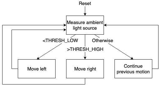
Following a similar approach, the algorithm for tracking a light source is implemented using the flowchart above. This algorithm explains why the robot moves toward the light source in a zig-zag fashion. Given the limitation of having only one onboard ambient light sensor, significant improvements to the algorithm are not feasible.
Results and Demonstration
The following parameters were used for this algorithm to move toward the direction of the light source:
- Number of samples = 300. To measure ambient light, we use the function
get_ambientlight()to read the current sensor value. If the sensor cannot return a good reading, it returns -1. Since these sensors are inherently noisy, a function is implemented to "sample" the current light level by averaging 300 sensor readings while discarding any bad sensor readings. THRESH_LOW= 300THRESH_HIGH= 600
A video demonstration of the problem statement can be accessed using the link below.

Different values for THRESH_LOW and THRESH_HIGH were chosen to implement hysteresis behavior, thereby preventing jittery motion. A high value of THRESH_HIGH ensures that the Kilobot moves closer to the light source. The function get_ambientlight() returns a 10-bit measurement (0 to 1023). The value of THRESH_HIGH can be adjusted to achieve better convergence toward the light source.
Synchronizing Phase of Blinking LEDs
In this section, we vreate a logical synchronous clock between different robots to allow two or more Kilobots to blink an LED in unison roughly every 4 seconds.
A large group of decentralized, closely cooperating entities, commonly called a collective or swarm, can work together to complete tasks beyond the capabilities of individuals. Kilobots have mastered the following three basic swarm behaviors:
- Foraging – Robots disperse and explore the surrounding area, reducing the time required to search a particular location.
- Formation Control – Kilobots can behave in unison or form specific structures within the swarm. They communicate with each other to maintain spatial awareness and coordination.
- Synchronization – Used to coordinate simultaneous actions among multiple robots or sensor networks. For example, a swarm of Kilobots could use LED lights to create a synchronized display, acting as pixels in a larger image.
Synchronization is an essential swarm behavior that enables coordinated actions between multiple robots.
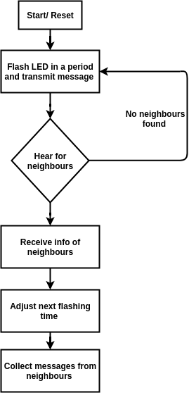
For this objective, an averaging-based synchronization method is used. Each Kilobot functions as an oscillator, blinking its LED at a fixed period P. Simultaneously, it transmits a message containing its current position in the clock cycle (a value between 0 and P). If there are no neighbors, the Kilobot blinks at a fixed period, like a firefly. If it detects neighboring Kilobots, it adjusts its flashing time based on the average received clock values.
Step 1: Create a Robot Oscillator
The Kilobot flashes every 2 seconds using the following code:
#define PERIOD 64
    uint32_t reset_time = 0;

    // In Program Loop
    if (kilo_ticks >= (last_reset + PERIOD)) {
       set LED to red;
       last_reset = kilo_ticks;
    } else {
       turn LED off;
    }
Step 2: Transmit the Current Clock Position
The Kilobot continuously transmits the current position of its clock within its ticking period (kilo_ticks - last_reset). Since the clock resets every 64 ticks, this value remains below 64.
message_t message;

    message_t *message_tx() {
        message.data[0] = kilo_ticks - last_reset; // current position in PERIOD
        message.crc = message_crc(&message);
        return &message;
    }
Step 3: Adjust the Clock Based on Neighboring Robots
When receiving a message from a neighbor, the Kilobot calculates the time difference and adjusts its next flashing time accordingly.
void message_rx(message_t *m, distance_measurement_t *d)
    {
        int my_timer = kilo_ticks - last_reset;
        int rx_timer = m->data[0];
        int timer_discrepancy = my_timer - rx_timer;

        // Reset time adjustment
        reset_time_adjustment = reset_time_adjustment + rx_reset_time_adjustment;
    }
Results and Demonstration
The following parameters were used for this synchronization algorithm:
- Period = 50. The Kilobot's internal clock uses
kilo_ticks, where one tick is approximately 30 ms, equating to around 32 ticks per second. - RESET_TIME_ADJUSTMENT_DIVIDER = 120. This value controls how much the Kilobot adjusts its reset time in response to discrepancies with neighbors. A larger value results in smaller adjustments and should be increased as the number of neighboring robots increases.
A video demonstration can be accessed using the link below.

Efficient Star-Planet Orbiting Using a Finite State Machine
Finite State Machine (FSM)
Before discussing FSM, let us discuss the three individual terms comprising this concept: finite, state, and machine. Finite refers to a fixed number, whereas state means the mode or position. For example, in the case of a traffic light signal, we have three different states: red, yellow, and green. Thus, FSM denotes a machine with a fixed number of states. A FSM can be viewed as:
- A set of input events
- A set of output events
- A set of states
- A function that maps states and input to output
- A function that maps states and inputs to states
- A description of the initial state
In the case of star-planet orbiting, we model the problem as an FSM, given its suitability for modularizing different components of the algorithm. Our mechanism for orbiting is very similar to those provided on the Kilobotics website, and elaborately covered in previous chapters. However, implementation using an FSM dramatically simplifies integrating macros of large size. Our main contribution in this chapter includes a novel and robust obstacle avoidance algorithm to prevent the planet from hitting the star if it starts too close to it, as well as a simple extension of the existing orbiting algorithm for a multiple stars setting. Both of these contributions will be discussed in the coming sections.
Flowchart
The flowchart for the orbit after escape algorithm is divided into two parts: Figure 1 and Figure 2. The first part discusses the extension of the orbit algorithm for a multiple star setting, while the latter illustrates the algorithm for escaping an obstacle.
Part I: Extension of Orbit Algorithm for Multiple Star Setting
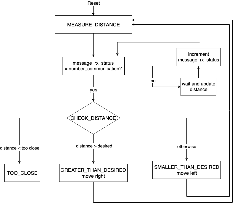
In the star-planet orbiting algorithm, while measuring the distance between stars and the planet, the parameter NUMBER_COMMUNICATION defines how many messages the planet should aggregate before making a decision. Accordingly, the planet identifies the nearest star based on the strength of the signal received in the previous step. Considering the nearest star, the planet either moves left or right to maintain DESIRED_DISTANCE. The parameter message_rx_status is used to keep count of successful communications.
Part II: Escaping Obstacle
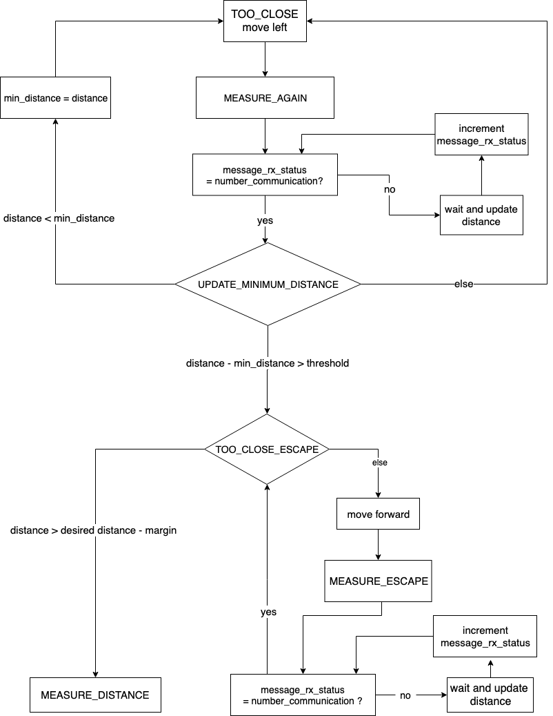
The parameter NUMBER_COMMUNICATION affects the speed of the planet. For example, if the number of stars in communication range is more, the planet moves faster than if it has only one star in communication range. This is because the planet needs to receive NUMBER_COMMUNICATION measurements from only one star before deciding the motion. The following observations demonstrate how the revolution time is affected by the number of communications:
- Motor delay = 200, Number of communications = 4, Revolution time = 23 minutes
- Motor delay = 500, Number of communications = 2, Revolution time = 5 minutes
While escaping from the TOO_CLOSE region, we compare successive distance measurements to check the orientation of the planet from the star. In an earlier version of the algorithm, we tried to detect the transition of distance from increasing to decreasing as the instant when the planet is oriented away from the star, but due to uncertainty in measurements, this led to unwanted behavior. Therefore, we decided to keep track of minimum_distance from the star and check the condition distance - min_distance > THRESHOLD_ROTATE. By appropriately choosing THRESHOLD_ROTATE, we were able to get the final orientation of the planet away from the direction of the star. Moreover, this modification reduced the dependence on the accuracy of a single measurement, resulting in a filter-like behavior and increased robustness.
It is worth mentioning that the robustness comes at an additional cost: in the worst-case scenario, the planet might require one complete revolution before being able to escape the TOO_CLOSE region of the star.
Results and Demonstration
The caption of Figure 3 provides a link to the demonstration for the orbiting of the planet around the star, given that the star starts near the desired distance.

We have hard delays in our current implementation, which increases the revolution time. In the future, these can be replaced with soft delays to alleviate the time of revolution.
The caption of Figure 4 provides a link to the demonstration of the algorithm for the planet to move away from the too-close region, which involves using a robust algorithm followed by orbiting.

It is evident from the demonstration that there is a damped oscillation before the planet starts orbiting. This can be attributed to differences in the center of rotation of Kilobots for clockwise and anti-clockwise turns. If it rotated about its center, the oscillations would not have been as pronounced as in the current scenario.
The caption of Figure 5 provides a link to the demonstration of the algorithm for the planet to orbit around two stars. In this case, only one communication was used to identify the minimum distance, leading to instability, which can be attributed to the CSMA/CD communication protocol followed by Kilobots.

The caption of Figure 6 provides a link to the demonstration of the algorithm for the planet to orbit around two stars where the planet uses two communications to make a decision (estimating the minimum distance).

The caption of Figure 7 provides a link to the demonstration of the algorithm for the planet to orbit around three stars forming a triangle. In this case, the planet uses four communications to make a decision. Though these four communications stabilize the movement of the planet, they also increase the total revolution time.

Conclusion
We implemented a robust algorithm for star-planet orbiting using the concepts of FSM. This algorithm was able to prevent the planet from hitting the star, even if the planet starts in a very close region of the star. Additionally, we observed that the movement of a planet can be stabilized by increasing the number of communications from the star. However, this also increases the total revolution time. Furthermore, the orientation of the planet and star plays a significant role. If the orientation of the planet is away from that of the star, it might take an additional turn before it begins orbiting.
Shape Formation Using Kilobots
In this chapter, we will discuss an algorithm motivated by the work of SSL lab, Harvard University, for shape formation. Rather than implementing the entire algorithm, we will only consider a portion of it, assuming that the next robot to be placed is available near the origin.
Framework
- Three robots (guides) are used as reference for axis orientation.
- A robot (builder) participating in shape formation starts near the left of the origin.
- In its effort to reach the desired location, the builder orbits around the partial shape using the algorithm presented in the previous chapter.
- The builder stops orbiting when it reaches the desired location.
- The builder becomes a guide, thereby helping the next builder.
To participate in shape formation, builders need to decide upon the global shape to form. This is achieved by sharing a shape matrix encapsulating the desired shape as an array of 5-tuple. The 5-tuple contains the following information necessary for establishing builders at desired locations:
(Index, Neighbour_1, Desired_distance_1, Neighbour_2, Desired_distance_2)
For forming a linear shape of width 2, the shape matrix would look like:
[3, 1, 1, 2, 1]
        [4, 2, 1, 3, √2]
        [5, 3, 1, 4, 1]
        [..., ..., ..., ..., ...]
It is important to note that we require the shape to ensure two guides for each builder node, or else the builder would fail to localize correctly.
Flowchart
Figure 1 explains the algorithm for shape formation. Our algorithm differs from the previous work in its implementation of the shape matrix and localization, which will be discussed later.

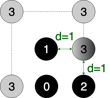
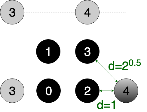
Discussion
Figures 2 and 3 help in visualizing the shape formation process for the shape matrix provided above, which corresponds to a line of width 2. Black circles indicate guide robots, which continuously transmit their Index, whereas grey circles indicate the oncoming builder robot. The shaded circle corresponds to a builder transforming into a guide. A builder is always in listener mode, whereas a guide is always in speaker mode of communication. Dotted lines trace the path of the builder.
When the first builder initialized with Index=3 starts its journey, it never faces a situation that requires an Index update and ultimately reaches the desired location corresponding to Index=3 and transforms into a guide robot.
When the second builder arrives with Index=3, as shown in Figure 3, it continues its journey to occupy the desired location corresponding to Index=3. However, when it comes into the communication range of the new guide with Index=3, it realizes that it needs to update its Index to 4. After this, it travels to the desired location corresponding to Index=4 and transforms into a guide.
Demonstration
EPSILON_MARGIN and MOTOR_ON_DURATION play an essential role in determining the stability and accuracy of shape formation. For a large MOTOR_ON_DURATION, it is likely that the builder will go beyond its desired location and continue orbiting, whereas for larger EPSILON_MARGIN, we get distortion in shape. Moreover, we cannot choose very small EPSILON_MARGIN due to measurement errors. One way to improve accuracy is by adaptively decreasing the MOTOR_ON_DURATION of the builder as it comes into the communication range of its desired neighbors.
The two parameters discussed are borrowed from the previous chapter. For detailed understanding of these parameters, readers are encouraged to refer to the code in Appendix C.
Based on our discussion, the inclusion of the following measures would boost the performance:
- Adaptively decreasing the
MOTOR_ON_DURATIONas the builder reaches closer to its target location. This would significantly improve the runtime of shape formation and accuracy of localization if calibrated with the proper choice ofEPSILON_MARGIN. - Conversion of hard delays to soft delays, thereby decreasing the overall run time.
- Use of optimization-based approaches for localization to incorporate uncertainty in measurements.
Documentation

Alternatively, one can refer to the presentation slides focused towards shape formation algorithm. It includes most of the building blocks required for shape formation followed by demonstration of individual blocks.
Acknowledgement
I would like to thank Sudhakar Kumar, Eswara Srisai, and Kishan Chouhan who, as a part of four member team, played an essential part in success of the project. This project was undertaken as a part of lab work (SC 626) under the guidance of Prof. Leena Vachhani and Prof. Arpita Sinha.
Author
Anurag Gupta is an M.S. graduate in Electrical and Computer Engineering from Cornell University. He also holds an M.Tech degree in Systems and Control Engineering and a B.Tech degree in Electrical Engineering from the Indian Institute of Technology, Bombay.
Comment
This policy contains information about your privacy. By posting, you are declaring that you understand this policy:
- Your name, rating, website address, town, country, state and comment will be publicly displayed if entered.
- Aside from the data entered into these form fields, other stored data about your comment will include:
- Your IP address (not displayed)
- The time/date of your submission (displayed)
- Your email address will not be shared. It is collected for only two reasons:
- Administrative purposes, should a need to contact you arise.
- To inform you of new comments, should you subscribe to receive notifications.
- A cookie may be set on your computer. This is used to remember your inputs. It will expire by itself.
This policy is subject to change at any time and without notice.
These terms and conditions contain rules about posting comments. By submitting a comment, you are declaring that you agree with these rules:
- Although the administrator will attempt to moderate comments, it is impossible for every comment to have been moderated at any given time.
- You acknowledge that all comments express the views and opinions of the original author and not those of the administrator.
- You agree not to post any material which is knowingly false, obscene, hateful, threatening, harassing or invasive of a person's privacy.
- The administrator has the right to edit, move or remove any comment for any reason and without notice.
Failure to comply with these rules may result in being banned from submitting further comments.
These terms and conditions are subject to change at any time and without notice.
Similar content


Past Comments